Logistic regression

Logistic regression can be used to estimate the probability of response based on one or more variables or features. It can be used to predict categorical response with multiple levels, but the post here focuses on binary response which we can call it binary logistic models. It will only take two kinds of responses, such as fail/pass, 0 or 1.

Logistic regression
Binary logistic regression from Scikit-learn
1. linear_model.LogisticRegression
2. Classification and prediction boundary
Binary logistic regression from scratch
Reference

Logistic regression takes the form of a logistic function with a sigmoid curve. The logistic function can be written as: $P(X)={\frac{1}{1+e^{-(\beta _{0}+\beta _{1}x_{1}+ \beta _{2}x_{2}+..)}}}$ where P(X) is probability of response equals to 1, $P(y=1)$ .

The post has two parts:

use Sk-Learn function directly
coding logistic regression prediction from scratch

Binary logistic regression from Scikit-learn

linear_model.LogisticRegression

Sk-Learn is a machine learning library in Python, built on Numpy, Scipy and Matplotlib. The post will use function linear_model.LogisticRegression from Sk-learn.

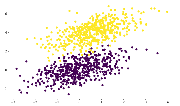
We will first simulate a dataset using bi-variate (two variables) normal distribution:

import matplotlib
import numpy as np
import matplotlib.pyplot as plt
%matplotlib inline
matplotlib.rcParams['figure.figsize'] = (10.0, 6.0)

np.random.seed(3)
num_pos = 5000

# Bivariate normal distribution mean [0, 0] [0.5, 4], with a covariance matrix
subset1 = np.random.multivariate_normal([0, 0], [[1, 0.6],[0.6, 1]], num_pos)
subset2 = np.random.multivariate_normal([0.5, 4], [[1, 0.6],[0.6, 1]], num_pos)

dataset = np.vstack((subset1, subset2))
labels = np.hstack((np.zeros(num_pos), np.ones(num_pos)))

plt.scatter(dataset[:, 0], dataset[:, 1], c=labels)
plt.show()

regression1

Then we can use linear_model.LogisticRegression to fit a model:

from sklearn import linear_model
clf = linear_model.LogisticRegression()
clf.fit(dataset, labels)
print(clf.intercept_, clf.coef_, clf.classes_)

[-8.47053414] [[-2.19855235  4.54589066]] [0 1]

The intercept $\beta_{0}=-8.4705$ , and two coefficients $\beta_{1}=-2.1985, \beta_{2}=4.5458$ . The fitted model can be used to predict new data point, such as $(x_{1}=0 , x_{2}=1), (x_{1}=1 , x_{2}=4)$ .

clf.predict_proba([[0, 0], [1, 4]])

array([[  9.99790491e-01,   2.09509039e-04],
       [  5.44838493e-04,   9.99455162e-01]])

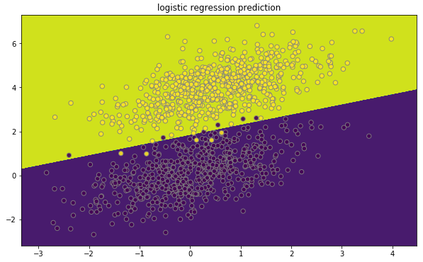
$\begin{align*} P(label=0|x_{1}=0 , x_{2}=1) = 99.97\% \\ P(label=1|x_{1}=1 , x_{2}=4) = 99.94\% \\ \end{align*}$

Classification and prediction boundary

We can systematically plot classification and its prediction boundary using the function below.

# it is a frequently used plot function for classification
def plot_decision_boundary(pred_func, X, y, title):
    # Set min and max values and give it some padding
    x_min, x_max = X[:, 0].min() - .5, X[:, 0].max() + .5
    y_min, y_max = X[:, 1].min() - .5, X[:, 1].max() + .5
    h = 0.01
    # Generate a grid of points with distance h between them
    xx, yy = np.meshgrid(np.arange(x_min, x_max, h), np.arange(y_min, y_max, h))
    # Predict the function value for the whole grid (get class for each grid point)
    Z = pred_func(np.c_[xx.ravel(), yy.ravel()])
    Z = Z.reshape(xx.shape)
    # print(Z)
    # Plot the contour and training examples
    plt.contourf(xx, yy, Z)
    plt.scatter(X[:, 0], X[:, 1], c=y, s=40, edgecolors="grey", alpha=0.9)
    plt.title(title)
    plt.show()

# run on the training dataset with predict function
plot_decision_boundary(lambda x: clf.predict(x), dataset,
                       labels, "logistic regression prediction")

regression2

Binary logistic regression from scratch

Linear algebra and linear regression

Numpy python library empowers the computation of multi-dimensional arrays and matrices. To speed up the calculation and avoid loops, we should formulate our computation in array/matrix format. Numpy provides both array and matrix, it is recommended using array type in Python since it is the basic type in Numpy. Many Numpy function return outputs as arrays, not matrices. The array type uses dot instead of * to multiply (reduce) two tensors. It might be a good idea to read the NumPy for Matlab users article.

For linear regression which is $Y=X\beta+\varepsilon$ , where $Y= \begin{pmatrix} y_{1}\\ y_{2}\\ \vdots \\ y_{n}\\ \end{pmatrix}$

$X= \begin{pmatrix} x_{1,1} & x_{1,2} & \cdots & x_{1,p} \\ x_{1,1} & x_{1,2} & \cdots & x_{1,p} \\ \vdots & \vdots & \ddots & \vdots \\ x_{n,1} & x_{n,2} & \cdots & x_{n,p} \\ \end{pmatrix}$

and

$\beta= \begin{pmatrix} \beta_{1}\\ \beta_{2}\\ \vdots \\ \beta_{p}\\ \end{pmatrix}$

if we write them in array type in Numpy, with np.shape(Y) = (n, 1), np.shape(X) = (n, p), np.shape( $\beta$ ) = (p, 1), it should use Y=np.dot(X, $\beta$ ). So we can initialize the data in Python code below:

import matplotlib
import numpy as np
import matplotlib.pyplot as plt

np.random.seed(3)
num_pos = 5000

# Bivariate normal distribution mean [0, 0] [0.5, 4], with a covariance matrix
subset1 = np.random.multivariate_normal([0, 0], [[1, 0.6],[0.6, 1]], num_pos)
subset2 = np.random.multivariate_normal([0.5, 4], [[1, 0.6],[0.6, 1]], num_pos)

dataset = np.vstack((subset1, subset2))
# add 1 for beta_0 intercept
x = np.hstack((np.ones(num_pos*2).reshape(num_pos*2, 1), dataset))
y = np.hstack((np.zeros(num_pos), np.ones(num_pos))).reshape(num_pos*2, 1)
beta = np.zeros(x.shape[1]).reshape(x.shape[1], 1)

# check shape
print(np.shape(y))
print(np.shape(x))
print(np.shape(beta))
print(np.shape(np.dot(x, beta)))

(10000, 1)
(10000, 3)
(3, 1)
(10000, 1)

Logistic regression function

Logistic regression takes the form of a logistic function with a sigmoid curve. The logistic function can be written as: $P(X)={\frac{1}{1+e^{-(\beta _{0}+\beta _{1}x_{1}+ \beta _{2}x_{2}+..)}}}={\frac{1}{1+e^{-X\beta}}}$ where P(X) is probability of response equals to 1, $P(y=1|X)$ , given features matrix X. We can call it $\hat{Y}$ , in python code, we have

x_beta = np.dot(x, beta)
y_hat = 1 / (1 + np.exp(-x_beta))

We can also reformulate the logistic regression to be logit (log odds) format which we can use as a trick for induction on derivative.

$log\left(\frac{P(X)}{1-P(X)}\right)=X\beta=\beta _{0}+\beta _{1}x_{1}+ \beta_{2}x_{2}+..$

Likelihood function

Likelihood is a function of parameters from a statistical model given data. The goal of model fitting is to find parameter (weight $\beta$ ) values that can maximize the likelihood.

The likelihood function of a binary (either 0 or 1) logistic regression with a given observations and their probabilities is

$\prod_{i=0}^N P_{i}^{y_{i}}(1-P_{i})^{1-y_{i}}$

The log likelihood of the model given a dataset/observations for ( $\beta$ ) is

$\begin{align} L(\beta) &= \sum_{i=0}^N \Bigl( y_{i}logP(x_{i})+(1-y_{i})log\bigl(1-P(x_{i})\bigl) \Bigl) & \text{take log of the product above } \\ &= \sum_{i=0}^N log\bigl( 1-P(x_{i}) \bigl) + \sum_{i=0}^N (y_{i}log\frac{P(x_{i})}{1-P(x_{i})}) & \text{regroup by $y_{i}$ }\\ &= \sum_{i=0}^N log\bigl( 1-P(x_{i}) \bigl) + \sum_{i=0}^N (y_{i} x_{i}\beta) & \text{ use the logit (log odds) }\\ \end{align}$

likelihood = np.sum(np.log(1 - y_hat)) + np.dot(y.T, x_beta)

Gradient

The goal of model fitting is to find parameter (weight $\beta$ ) values that maximize the likelihood, or maximum likelihood estimation (MLE) in statistics. We can use the gradient ascent as a general approach. The log-likelihood is the function of $\beta$ and gradient is the slope of the function at the current $\beta$ position. The gradient not only shows the direction we should increase the values of $\beta$ which increase the log-likelihood, but also the step size we should increase $\beta$ . When the slope is large, we should increase $\beta$ more (take bigger step) towards the the maximum.

The gradient here can use the derivative of log-likelihood function with respect to each parameter $\beta_{j}$ , $\frac{\partial{L}}{\partial{\beta_{j}}}$ . For the second summation, it is easy and we can get $\frac{\partial{y_{i} x_{i}\beta}}{\partial{\beta_{j}}}=y_{i} x_{ij}$

For the first summation with P( $x_{i}$ ), we first use a nice property of $P(X)$ . If we make $z_{i}=x_{i}\beta$ , then

$\begin{align} P(x_{i}) &= \frac{1}{1+e^{-x_{i}\beta}}=\frac{1}{1+e^{-z_{i}}}=P(z_{i})=\frac{e^{z_{i}}}{1+e^{z_{i}}}\\ \frac{\partial{P(z_{i})}}{\partial{z_{i}}} &= \frac{e^{z_{i}}}{1+e^{z_{i}}}+e^{z_{i}}(-1)(1+e^{z_{i}})^{-2}e^{z_{i}}=\frac{1}{1+e^{z_{i}}}\frac{e^{z_{i}}}{1+e^{z_{i}}}=P(z_{i})\bigl(1-P(z_{i})\bigl)\\ \frac{\partial{P(x_{i})}}{\partial{\beta_{j}}} &= \frac{\partial{P(z_{i})}}{\partial{z_{i}}}\frac{\partial{z_{i}}}{\partial{\beta_{j}}}=P(z_{i})\bigl(1-P(z_{i})\bigl)\frac{\partial{x_{i}\beta}}{\partial{\beta_{j}}}=P(x_{i})\bigl(1-P(x_{i})\bigl)x_{ij}\\ \end{align}$

The last equation above is a nice property we will use in the next step. Now, we have

$\frac{ \partial{log\bigl( 1-P(x_{i}) \bigl)} }{\partial{\beta_{j}}}=\frac{1}{1-P(x_{i})}(-1)\frac{\partial{P(x_{i})}}{\partial{\beta_{j}}}=-P(x_{i})x_{ij}$

$\frac{\partial{L}}{\partial{\beta_{j}}}=\sum_{i=0}^N \bigl( y_{i}x_{ij} - P(x_{i})x_{ij} \bigl)=\sum_{i=0}^N \bigl( y_{i} - P(x_{i}) \bigl)x_{ij}$

, where $P(x_{i})$ is $\hat{Y}$ , the prediction of $y$ based on $x$ . So the gradient is

gradient = np.dot(np.transpose(x), y - y_hat)

Use the gradient to update the $\beta$ array with $\Delta{\beta}$ , and a small learning rate

beta = beta + learning_rate * gradient

The learning rate is step size moving the likelihood towards maximum:

gradient ascent beta in likelihood 2D

Full script

Finally, we get everything ready, with

Training data, features X and observations Y
Initial values for weights ( $\beta$ )
Ways to calculate gradient, and update weights ( $\beta$ )

We can run multiple iterations and gradually update weights to approach the maximum of likelihood. Script below also contains a repeat run using Sklearn which shows almost the same estimation of weights ( $\beta$ ) given the same training dataset.

Code:

import matplotlib
import numpy as np
import matplotlib.pyplot as plt

np.random.seed(3)
num_pos = 5000
learning_rate = 0.0001
iterations = 50000

# Bivariate normal distribution mean [0, 0] [0.5, 4], with a covariance matrix
subset1 = np.random.multivariate_normal([0, 0], [[1, 0.6],[0.6, 1]], num_pos)
subset2 = np.random.multivariate_normal([0.5, 4], [[1, 0.6],[0.6, 1]], num_pos)

dataset = np.vstack((subset1, subset2))
x = np.hstack((np.ones(num_pos*2).reshape(num_pos*2, 1), dataset)) # add 1 for beta_0 intercept
label = np.hstack((np.zeros(num_pos), np.ones(num_pos)))
y = label.reshape(num_pos*2, 1) # reshape y to make 2D shape (n, 1)
beta = np.zeros(x.shape[1]).reshape(x.shape[1], 1)

for step in np.arange(iterations):
    x_beta = np.dot(x, beta)
    y_hat = 1 / (1 + np.exp(-x_beta))
    likelihood = np.sum(np.log(1 - y_hat)) + np.dot(y.T, x_beta)
    preds = np.round( y_hat )
    accuracy = np.sum(preds == y)*1.00/len(preds)
    gradient = np.dot(np.transpose(x), y - y_hat)
    beta = beta + learning_rate*gradient
    if( step % 5000 == 0):
        print("After step {}, likelihood: {}; accuracy: {}"
              .format(step+1, likelihood, accuracy))


print(beta)

# compare to sklearn
from sklearn import linear_model
# Logistic regression class in sklearn comes with L1 and L2 regularization,
# C is 1/lambda; setting large C to make the lamda extremely small
clf = linear_model.LogisticRegression(C = 100000000, penalty="l2")
clf.fit(dataset, label)
print(clf.intercept_, clf.coef_)

After step 1, likelihood: [[-6931.4718056]]; accuracy: 0.5
After step 5001, likelihood: [[-309.43671144]]; accuracy: 0.9892
After step 10001, likelihood: [[-308.96007441]]; accuracy: 0.9893
After step 15001, likelihood: [[-308.94742145]]; accuracy: 0.9893
After step 20001, likelihood: [[-308.94702925]]; accuracy: 0.9893
After step 25001, likelihood: [[-308.94702533]]; accuracy: 0.9893
After step 30001, likelihood: [[-308.94702849]]; accuracy: 0.9893
After step 35001, likelihood: [[-308.94701465]]; accuracy: 0.9893
After step 40001, likelihood: [[-308.94701912]]; accuracy: 0.9893
After step 45001, likelihood: [[-308.94702355]]; accuracy: 0.9893

[[-10.20181874]
 [ -2.64493647]
 [  5.4294686 ]]
[-10.17937262] [[-2.63894088  5.41747923]]

Note, sklearn.linear_model.LogisticRegression comes with regularization, which use L1 or L2 norm penalty, to prevent model over fitting. The option C is the inverse of regularization strength. Smaller values specify stronger regularization. Here, we use an extremely large C number to eliminate the L1 or L2 norm penalty, so the weights ( $\beta$ ) will be estimated in the same way as we programmed from scratch.

Machine Learning in Python - Logistic Regression

Tags