TensorFlow has been a popular tool in machine learning since Google decided to open source the library. The software is using graph based computation. Unlike regular computations in Python and R where analyses are carried out sequentially, TensorFlow first constructs a graph based on placeholders and variables then do the computations in parallel across CPUs or GPUs with data feeds. Google also creates their own processing unit called TPU which is available to on their cloud platform.
Table of Contents
I will introduce the TensorFlow with a few of examples from hello word to neural network. As usual, I prepared my codes sequentially without packaging them into functions. It would be more straightforward to readers.
Hello world
The script below is a “hello world” example using TensorFlow. It first creates a constant node in the graph. When the Tensoflow runs a session, the value is returned from the constant construction.
import sys
import tensorflow as tf
hello = tf.constant('Hello, TensorFlow!')
sess = tf.Session()
print(sess.run(hello))
b'Hello, TensorFlow!'
Basic operations
The script below first defines two placeholders, a and b, with data type int16. They are placeholders without any value assigned. Then a graph is being constructed with add, multiply operations. The two operations can be run in parallel since they are not relying on each other. Another layer of add operation is added on top which will be run after two parallel operations are finished. The tf.session fires a run on the graph with data feeds for placeholder a and b.
import sys
import tensorflow as tf
a = tf.placeholder(tf.int16)
b = tf.placeholder(tf.int16)
add = tf.add(a, b)
mul = tf.multiply(a, b)
final = tf.add(add, mul)
with tf.Session() as sess:
    o1, o2, o3 = sess.run([add, mul, final], feed_dict={a: 2, b: 3})
    print("add: {}; multiply: {}; final: {}".format(o1, o2, o3))
add: 5; multiply: 6; final: 11
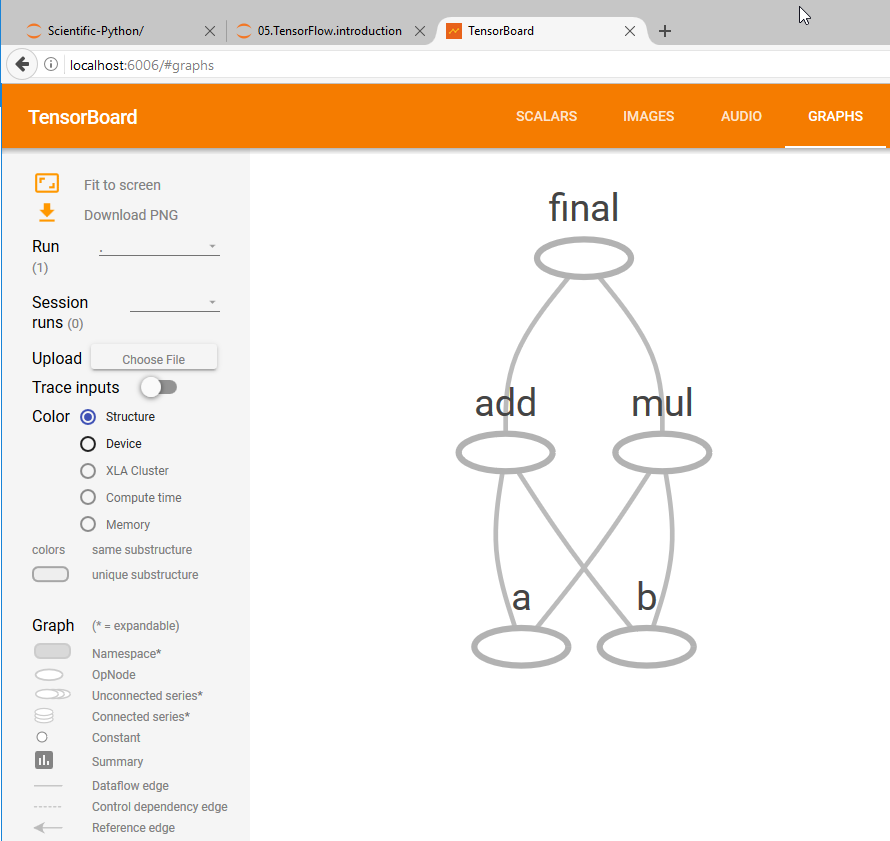
TensorFlow also offers a learning visualizing tool, TensorBoard, where user can visualize TensorFlow graph and plot quantitative metrics. If we add name to each operation node to the script above:
import sys
import tensorflow as tf
import os
cwd = os.getcwd()

a = tf.placeholder(tf.int16, name="a")
b = tf.placeholder(tf.int16, name="b")
add = tf.add(a, b, name="add")
mul = tf.multiply(a, b, name="mul")
final = tf.add(add, mul, name="final")
with tf.Session() as sess:
    writer = tf.summary.FileWriter("output", sess.graph)
    o1, o2, o3 = sess.run([add, mul, final], feed_dict={a: 2, b: 3})
    writer.close()
    print("add: {}; multiply: {}; final: {}".format(o1, o2, o3))
    print("run TensorBoard in "+cwd)
add: 5; multiply: 6; final: 11
run TensorBoard in C:\Documents\path\to\workdir
The writer will generate a file with name “events.out.tfevents.xxxxxx” in the “output” folder. Run the following command in CMD (Windows) or Terminal (Linux/Mac):
cd C:\Documents\path\to\workdir
tensorboard --logdir="output"
Starting TensorBoard b'54' at http://localhost:6006
(Press CTRL+C to quit)
Here, I noticed one issue. The TensorBoard graph will not showing if we use absolute path in “–logdir”. It is working well with a relative path. Open a web browser:
Linear regression estimation
The script below first defines two placeholders: and ; two variable: and . The linear model graph is built based on
y_hat = tf.add(tf.multiply(x, w), b, name="pred")
The cost function to minimize can be defined as mean of squared error
loss = tf.reduce_mean(tf.pow(y - y_hat, 2))
TensorFlow provides a few of optimizers and we can use them directly without deriving gradient ourselves. It is automatically doing forward feeding and back propagation. For linear regression fit, we can use GradientDescentOptimizer function:
optimizer = tf.train.GradientDescentOptimizer(learning_rate=0.01).minimize(loss)
We are running gradient descent optimization by feeding each data point in a stochastic manner.
import numpy as np
import tensorflow as tf
import matplotlib.pyplot as plt
import matplotlib
%matplotlib inline
matplotlib.rcParams['figure.figsize'] = (12.0, 9.0)
np.random.seed(3)
n_samples=50
xbatch = np.random.random(n_samples)
ybatch=2.5*xbatch + 1.6 + np.random.normal(1, 0.3, n_samples)
n_samples = xbatch.shape[0]
# construct tf graph
# None allows x/y to take any number of samples
x = tf.placeholder(tf.float32, name="x") # input variables and bias term
y = tf.placeholder(tf.float32, name="y") # output for each input pair
# construct/initialize operation weights
w = tf.Variable(0.0, name="weights")
b = tf.Variable(0.0, name="bias")
# get y prediction using logistic regression
y_hat = tf.add(tf.multiply(x, w), b, name="pred")
# Define the loss as the mean squared error
loss = tf.reduce_mean(tf.pow(y - y_hat, 2))
# Minimize cost with Gradient Descent
optimizer = tf.train.GradientDescentOptimizer(learning_rate=0.01).minimize(loss)
# Testing a dataset
init = tf.global_variables_initializer()
# Launch the graph
with tf.Session() as sess:
sess.run(init)
#for i in np.arange(int(2*num_pos/mini_batchsize)):
for epoch in range(200):
for (xi, yi) in zip(xbatch, ybatch):
sess.run(optimizer, feed_dict={x: xi, y: yi})
if((epoch+1) % 20 == 0):
wi, bi = sess.run([w, b])
loss_i = sess.run(loss, feed_dict={x: xbatch, y: ybatch})
print("w:{0:.4f} b:{1:.4f} prediction loss: {2:.4f}"
.format(wi, bi, loss_i))
wi, bi = sess.run([w, b])
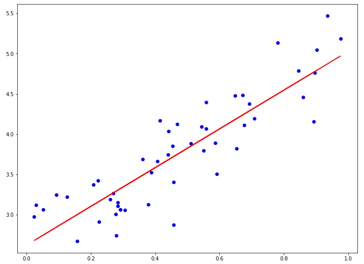
# plot the regression lines with training data points
plt.scatter(xbatch, ybatch, c="blue")
abline_values = [wi*i + bi for i in xbatch]
plt.plot(xbatch, abline_values, c="red")
plt.show()
w:2.0933 b:2.7750 prediction loss: 0.1152
w:2.2972 b:2.6744 prediction loss: 0.1095
w:2.3685 b:2.6393 prediction loss: 0.1087
w:2.3934 b:2.6270 prediction loss: 0.1086
w:2.4021 b:2.6227 prediction loss: 0.1086
w:2.4052 b:2.6211 prediction loss: 0.1086
w:2.4063 b:2.6206 prediction loss: 0.1086
w:2.4066 b:2.6204 prediction loss: 0.1086
w:2.4068 b:2.6204 prediction loss: 0.1086
w:2.4068 b:2.6203 prediction loss: 0.1086
Logistic regression classifier
In this section, we will rewrite the logistic regression classifier example in previous post using TensorFlow. In additional to linear regression setup above, the final prediction is using sigmoid transformation of linear regression out. It provides non-linear transformation and results in values in between 0 and 1.
For the cost function, although we can use squared error as we did for linear regression above, it is better to use TensorFlow’s sigmoid_cross_entropy_with_logits function directly.
I shuffled the data and create small batches with batch size 10. It will run 20 steps to go over all data point in each epoch. An epoch usually means one iteration over all the training data. I ran 500 epochs, and print out cost/accuracy at the end of every 50 epochs. To speed up the run, user can further shuffle around the dataset between epochs. Then they can speed up the training with less data input in each epoch.
import numpy as np
import tensorflow as tf
import matplotlib.pyplot as plt
import matplotlib
%matplotlib inline
matplotlib.rcParams['figure.figsize'] = (12.0, 9.0)

np.random.seed(5)
# construct tf graph
# None allows x/y to take any number of samples
x = tf.placeholder(tf.float32, [None, 2]) # two input variables and bias term
y = tf.placeholder(tf.float32, [None, 1]) # one output for each input pair

# construct/initialize operation weights
w = tf.Variable(tf.truncated_normal([2,1], stddev=0.1))
b = tf.Variable(tf.ones([1]))

# get y prediction using logistic regression
z = tf.matmul(x, w) + b
y_hat = tf.sigmoid(z)

# use this entry directly
cost = tf.reduce_sum(tf.nn.sigmoid_cross_entropy_with_logits(logits=z, labels=y))

# Or define the cost as the mean squared error
# cost = tf.reduce_mean(tf.pow(y - y_hat, 2))

# get accuracy definition
check = tf.cast(tf.equal(tf.round(y_hat), y), tf.float32) # convert True/False to 1/0
accuracy = tf.reduce_mean(check)

# Minimize cost with Gradient Descent
optimizer = tf.train.GradientDescentOptimizer(learning_rate = 0.01).minimize(cost)

# Testing a dataset
num_pos = 100

# Bivariate normal distribution mean [0, 0] [0.5, 4], with a covariance matrix
subset1 = np.random.multivariate_normal([0, 0], [[1, 0.6],[0.6, 1]], num_pos)
subset2 = np.random.multivariate_normal([0.5, 4], [[1, 0.6],[0.6, 1]], num_pos)

xbatch = np.vstack((subset1, subset2))
label = np.hstack((np.zeros(num_pos), np.ones(num_pos)))
ybatch = label.reshape(num_pos*2, 1)

# randomize so each batch looks similar
randomize = np.arange(num_pos*2)
np.random.shuffle(randomize)
xbatch = xbatch[randomize, :]
ybatch = ybatch[randomize, :]

# Initializing the variables
init = tf.global_variables_initializer()

mini_batchsize = 10
# Launch the graph
with tf.Session() as sess:
    sess.run(init)
    for epoch in range(500):
        for i in np.arange(int(2*num_pos/mini_batchsize)):
            batchbeg =  i*mini_batchsize
            batchend =  (i + 1)*mini_batchsize
            sess.run(optimizer, feed_dict={x: xbatch[batchbeg:batchend, :],
                     y: ybatch[batchbeg:batchend, :]})

        if((epoch+1) % 50 == 0):
            costi = cost.eval(feed_dict={x: xbatch, y: ybatch})
            acc_i = accuracy.eval(feed_dict={x: xbatch, y: ybatch})
            print("prediction loss: {0:.4f}, accuracy: {1:.4f}"
                  .format(costi, acc_i))

    w_pred, b_pred = sess.run([w, b])

print(w_pred, b_pred)
prediction loss: 11.4159, accuracy: 0.9850
prediction loss: 8.3163, accuracy: 0.9900
prediction loss: 7.1168, accuracy: 0.9950
prediction loss: 6.4532, accuracy: 0.9950
prediction loss: 6.0229, accuracy: 0.9950
prediction loss: 5.7174, accuracy: 0.9950
prediction loss: 5.4872, accuracy: 0.9950
prediction loss: 5.3066, accuracy: 0.9950
prediction loss: 5.1603, accuracy: 0.9950
prediction loss: 5.0390, accuracy: 0.9950
[[-2.51026034]
 [ 4.23945332]] [-7.9543128]
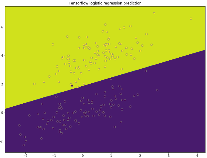
In the last step of the TensorFlow training, I printed out prediction for weights and bias, before session close in the “with” statement. We can then use the similar script we had in previous post to plot the prediction boundary.
x_min, x_max = xbatch[:, 0].min() - .5, xbatch[:, 0].max() + .5
y_min, y_max = xbatch[:, 1].min() - .5, xbatch[:, 1].max() + .5
h = 0.01
# Generate a grid of points with distance h between them
xx, yy = np.meshgrid(np.arange(x_min, x_max, h), np.arange(y_min, y_max, h))
X = np.vstack( ( xx.reshape(1, np.product(xx.shape)), yy.reshape(1, np.product(yy.shape)) ) ).T
# Predict the function value for the whole grid
zz = np.dot(X, w_pred) + b_pred
y_hat = 1 / (1 + np.exp(-zz))
pred = np.round(y_hat)
Z = pred.reshape(xx.shape)
# Plot the contour and training examples
plt.contourf(xx, yy, Z)
plt.scatter(xbatch[:, 0], xbatch[:, 1], c=ybatch, s=40, edgecolors="grey", alpha=0.9)
plt.title("Tensorflow logistic regression prediction")
plt.show()
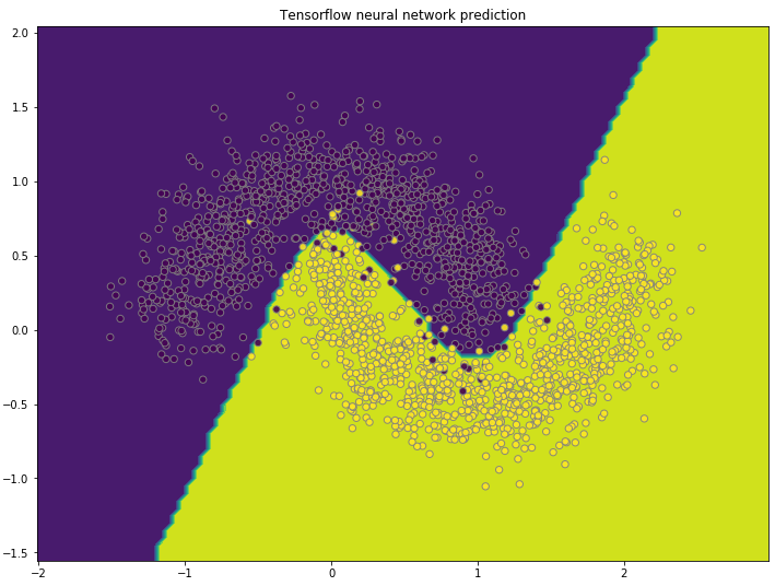
Neural network
In this section, we will rewrite the neural network classification on moon dataset in previous post using TensorFlow. The placeholder for x, and y using None for the first shape dimension so it can accept any number of samples as input for and . Same as the previous post, one hidden layer with three nodes is created, and only one node in the output layer. After linear combination, we used sigmoid’s nonlinearity and use TensorFlow’s sigmoid_cross_entropy_with_logits function as cost function directly.
When checking the accuracy, we directly convert True/False to 1.0/0.0 using tf.cast function.
During the training, it will go through all training data with batch size = 50 samples in each epoch. I ran 500 epochs, and print out cost/accuracy at the end of every 50 epochs.
import numpy as np
import tensorflow as tf
import matplotlib.pyplot as plt

# construct tf graph
# None allows x/y to take any number of samples
x = tf.placeholder(tf.float32, [None, 2]) # two input variables and bias term
y = tf.placeholder(tf.float32, [None, 1]) # one output for each input pair

# weights connecting the input to the hidden layer
w1 = tf.Variable(tf.truncated_normal([2,3], stddev=0.1))
b1 = tf.Variable(tf.zeros([1, 3]))

# weights connecting the hidden to the output layer
w2 = tf.Variable(tf.truncated_normal([3,1], stddev=0.1))
b2 = tf.Variable(tf.zeros([1, 1]))

# setup linear algebra and activate function for hidden layer
z1 = tf.add(tf.matmul(x, w1), b1)
h1 = tf.nn.sigmoid(z1)

# setup linear algebra and activate function for output node and final prediction
z2 = tf.add(tf.matmul(h1, w2), b2)
y_hat = tf.nn.sigmoid(z2)

# Define the cost as the mean squared error
cost = tf.reduce_sum(tf.nn.sigmoid_cross_entropy_with_logits(logits=z2, labels=y))

# get accuracy definition
check = tf.cast(tf.equal(tf.round(y_hat), y), tf.float32) # convert True/False to 1/0
accuracy = tf.reduce_mean(check)

# Minimize cost with Gradient Descent
optimizer = tf.train.GradientDescentOptimizer(learning_rate = 0.01).minimize(cost)

# Testing a dataset
# get file: https://github.com/welcomege/Scientific-Python/blob/master/data/moon_data.csv
moondata = np.genfromtxt('C:\\Documents\\Scientific-Python\\data\\moon_data.csv', delimiter=',')

nsample = np.shape(moondata)[0]
xbatch = moondata[:,1:3]
ybatch = moondata[:,0].reshape(nsample, 1)
# Initializing the variables
init = tf.global_variables_initializer()
mini_batchsize = 50

# Launch the graph
with tf.Session() as sess:
    sess.run(init)
    for epoch in range(500):
        for i in np.arange(int(nsample/mini_batchsize)):
            batchbeg =  i*mini_batchsize
            batchend =  (i + 1)*mini_batchsize
            sess.run(optimizer, feed_dict={x: xbatch[batchbeg:batchend, :],
                                           y: ybatch[batchbeg:batchend, :]})

        if((epoch+1) % 50 == 0):
            costi = cost.eval(feed_dict={x: xbatch, y: ybatch})
            acc_i = accuracy.eval(feed_dict={x: xbatch, y: ybatch})
            print("prediction loss: {0:.4f}, accuracy: {1:.4f}"
                  .format(costi, acc_i))

    w1_pred, b1_pred, w2_pred, b2_pred = sess.run([w1, b1, w2, b2])

#print(np.hstack((yh_i, ybatch, check_i)))
print(w1_pred, b1_pred, w2_pred, b2_pred)
prediction loss: 560.0883, accuracy: 0.8785
prediction loss: 555.5593, accuracy: 0.8790
prediction loss: 549.3909, accuracy: 0.8775
prediction loss: 541.3295, accuracy: 0.8785
prediction loss: 181.4227, accuracy: 0.9765
prediction loss: 144.8113, accuracy: 0.9760
prediction loss: 137.7171, accuracy: 0.9770
prediction loss: 134.9601, accuracy: 0.9770
prediction loss: 133.3959, accuracy: 0.9770
prediction loss: 132.3261, accuracy: 0.9770
[[-8.30357456  6.36264133  5.90656948]
 [ 3.88548803 -3.02339125  4.58996248]] [[-4.08502913 -8.24558163 -3.96620727]] [[-11.73311043]
 [ 12.85384655]
 [-11.4256649 ]] [[ 5.63598728]]
In the last step of the TensorFlow training, I printed out prediction for two weights and bias, before session close in the “with” statement. We can use the similar script we had in previous post to plot the prediction boundary:
- Get grid points with span=0.05
- Run the neural network forward feed with as input, and get prediction
- Plot the contour using , and prediction class.
- Plot the scatter points for training data points
x_min, x_max = xbatch[:, 0].min() - .5, xbatch[:, 0].max() + .5
y_min, y_max = xbatch[:, 1].min() - .5, xbatch[:, 1].max() + .5
h = 0.05
# Generate a grid of points with distance h between them
xx, yy = np.meshgrid(np.arange(x_min, x_max, h), np.arange(y_min, y_max, h))
X = np.vstack( ( xx.reshape(1, np.product(xx.shape)),
                 yy.reshape(1, np.product(yy.shape)) ) ).T
# Predict the function value for the whole grid
z1 = np.dot(X, w1_pred)+b1_pred
h1 = 1 / (1 + np.exp(-z1))
z2 = np.dot(h1, w2_pred)+b2_pred
y_hat = 1 / (1 + np.exp(-z2))
pred = np.round(y_hat)
Z = pred.reshape(xx.shape)
# Plot the contour and training examples
plt.contourf(xx, yy, Z)
plt.scatter(xbatch[:, 0], xbatch[:, 1], c=ybatch, s=40,
                          edgecolors="grey", alpha=0.9)
plt.title("Tensorflow neural network prediction")
plt.show()