Overview
In this post, we are going to implement a neural network from scratch in Python, and use it to classify a moon dataset.
Table of Contents
In the latest review paper authored by DeepMind’s co-founder, Demis Hassabis, he emphasized the importance of neuroscience as a rich source of inspiration of building deep learning and AI. “As the moniker ‘neural network’ might suggest, the origins of these AI methods lie directly in neuroscience. Ref
To mimic the neuron in brain, original data are weighted differently as inputs for different neuron node. Each neuron node receives signals from multiple inputs (just the same as dendrites in neural cell), and signals are summed and check against a certain threshold. If the accumulated signal is high enough, the neuron will fire and pass the signal to the downstream neurons. The process is:
- weight input values;
- sum signals from multiple input;
- activate neuron with an activation function.
The first two steps can be formulated as linear combination as we learn in linear algebra and last step can use activation function such as sigmoid and rectified linear unit (ReLU).
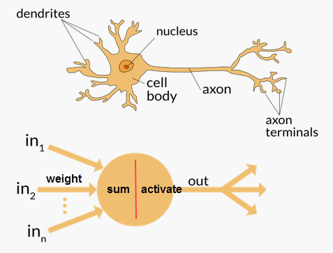
Neuroscience as a rich source of inspiration of building deep learning. Modified based on source
The post is not going to use Google’s Tensorflow library (the next post will), but you will get a good sense about Neural Network by playing a few examples in the Tensorflow playground site:
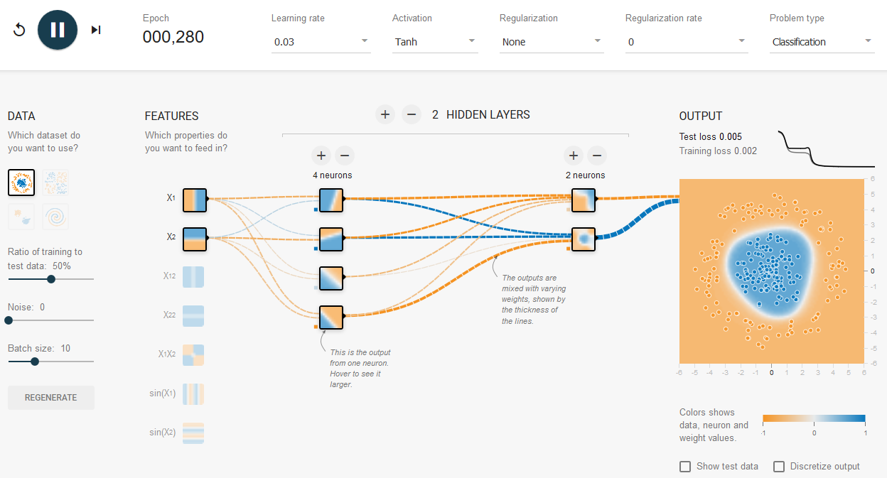 Tensorflow playground
Moon Dataset
Import the moon dataset from a csv file and plot
import numpy as np
import matplotlib.pyplot as plt
%matplotlib inline
matplotlib.rcParams['figure.figsize'] = (12.0, 9.0)

# https://github.com/welcomege/Scientific-Python/blob/master/data/moon_data.csv
moondata = np.genfromtxt('.\\data\\moon_data.csv', delimiter=',')

nsample = np.shape(moondata)[0]
x = moondata[:,1:3]
y = moondata[:,0].reshape(nsample, 1)
print(np.shape(moondata))
print(np.shape(x))
print(np.shape(y))
plt.scatter(x[:,0], x[:,1], c=y)
plt.show()
(2000, 3)
(2000, 2)
(2000, 1)
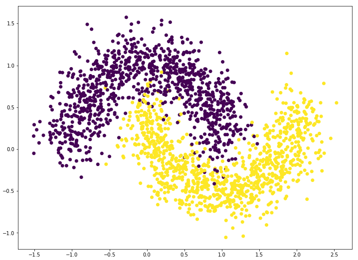 Moon data with two categories
The training/prediction using logistic regression will not achieve high accuracy on this moon data due to its non-linear pattern.
Build neural network model
In the moon dataset, there are two variables and , and a final prediction with value 0 or 1. We are going to build a simple model with two input variables and a bias term.
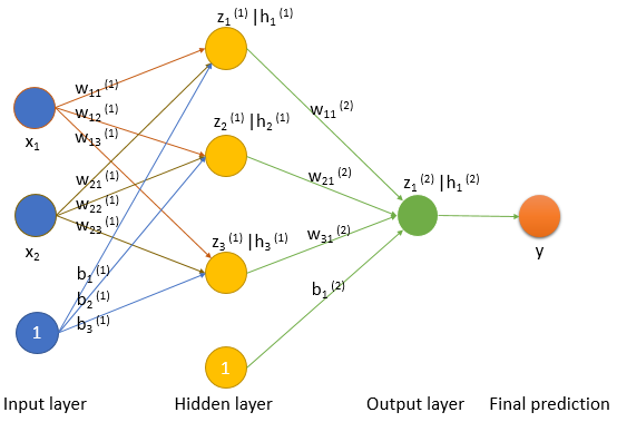
Neural network model
The linear combination of and will generate three neural nodes in the hidden layer. Note, we use to indicate layers: (1) to indicate first layer (hidden layer here), and will use (2) to indicate second layer (output layer).
Or write them in matrix form: , where is 2000 by 2 from input moon data, is 2 by 3, is 1 by 3, and is 2000 by 3.
We will choose the sigmoid function as an activation function:
, where is between 0.0 to 1.0 which can serve as a probability value for our prediction or .
The linear combination of values from three neural nodes and a bias term will generate the final output node. The prediction will be based on probability generated by sigmoid transformation of the final node.
Or write it in matrix form: , where is 20003 from input moon data, is 31, is 11, and is 20001.
after sigmoid function transformation, the model predict is 0 if and is 1 if
Code for feed-forward steps
The feed forward steps can be coded in following python code:
np.random.seed(3)

def f(z):
    return 1 / (1 + np.exp(-z))

n_hidden_node = 3
n_output_node = 1
# initilize with random numbers for weight and bias matrix
w1 = np.random.randn(2, n_hidden_node)
b1 = np.zeros((1, n_hidden_node))
w2 = np.random.randn(n_hidden_node, n_output_node)
b2 = np.zeros((1, n_output_node))

# forward propagation
z1 = np.dot(x, w1) + b1
h1 = f(z1)
z2 = np.dot(h1, w2) + b2
h2 = f(z2)

print("--------- x ---------")
print(x[0, :])
print("------- w1 & b1 -------")
print(w1, b1)
print("------- z1&h1 -------")
print(z1[0, :], h1[0, :])
print("------- w2&b2 -------")
print(w2, b2)
print("------- z2&h2 -------")
print(z2[0, :], h2[0, :])
print("--------- y ---------")
print(y[0, :])
--------- x ---------
[ 0.61065138 -0.45964566]
------- w1&b1 -------
[[ 1.78862847  0.43650985  0.09649747]
 [-1.8634927  -0.2773882  -0.35475898]] [[ 0.  0.  0.]]
------- z1&h1 -------
[ 1.94877477  0.39405562  0.22198974] [ 0.87531298  0.59725863  0.55527064]
------- w2&b2 -------
[[-0.08274148]
 [-0.62700068]
 [-0.04381817]] [[ 0.]]
------- z2&h2 -------
[-0.4712372] [ 0.38432346]
--------- y ---------
[ 1.]
For better illustration, put these numbers into neural graph:
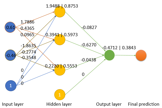
Example calculation:
0.61*1.7886-0.46*(-1.8635) + 1*0 = 1.9488
1/(1+exp(-1.9488)) = 0.8753
0.8753*(-0.0827) + 0.5973*(-0.6270) + 0.5553*(-0.0438) = -0.4712
1/(1+exp(0.4712)) = 0.3843
The first data point with , has produced which is far from the know true . It is expected since we did not do anything other than random guessing. Parameters in the neural network will be adjusted through back propagation in iterations until achieving good prediction.
Cost function and back propagation
In logistic regression post, the goal there was to maximize the log-likelihood. Weights/coefficients were updated using gradient ascent rules based on derivatives for each parameter. Here, to improve the model, we first define the objective, or cost function. The goal here is to accurately predict y using , or minimize the half mean squared error (hMSE):
We add ½ to the MSE cost function so that 2s are cancelled out when we take derivative. The cost function is a function of h, or cascade to inner hidden layers to be a function of weights and bias. We can derive the gradient based on derivative of MSE against each weight/bias, which is the slope of the cost function at current weight/bias position. The gradient not only shows the direction we should decrease the values of w/b which decrease the cost, but also the step size we should decrease weights. When the slope is large, we should decrease weights more (take bigger step) towards the minimum of MSE.
From output to hidden layer
First, we note hMSE as a function of ,
We first use derivative chain rule to back propagate the derivative of to derivative of . There is a useful property of sigmoid function we will use:
Here
Then
Because
Then we back propagate to weights and bias between hidden and output layer:
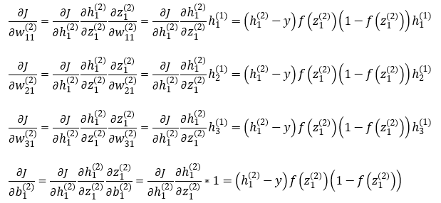
Before we propagate to inner layers, we first simply differential equation above using for layer :
Then
From hidden layer to input layer
Now we further back propagate to weights between input and inner layer, where
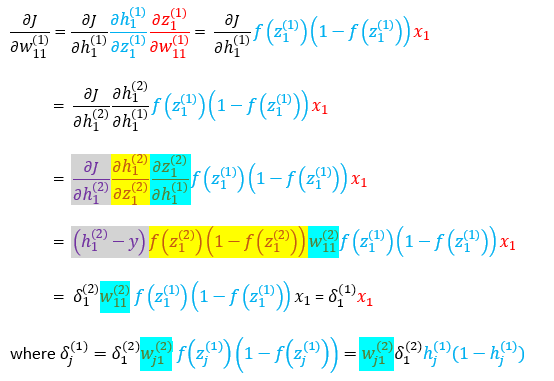
In the same way, we can get
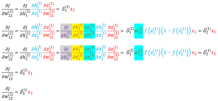
As we shown above, the back propagate is passing to with weight on the connection, and will be used to get :
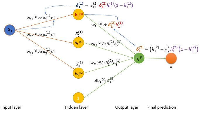
Back propagation code
For 2000 data point in the csv file,
- , where is from input moon data, is , is , and is .
- , where is from input moon data, is , is , and is .
Example of weights on initialization:
print("------- w1&w2 -------")
print(w1)
print(w2)
print("-- shape: w1&w2 -----")
print(np.shape(w1))
print(np.shape(w2))
print("------- b1&b2 -------")
print(b1)
print(b2)
print("-- shape: b1&b2 -----")
print(np.shape(b1))
print(np.shape(b2))
------- w1&w2 -------
[[ 1.78862847  0.43650985  0.09649747]
 [-1.8634927  -0.2773882  -0.35475898]]
[[-0.08274148]
 [-0.62700068]
 [-0.04381817]]
-- shape: w1&w2 -----
(2, 3)
(3, 1)
------- b1&b2 -------
[[ 0.  0.  0.]]
[[ 0.]]
-- shape: b1&b2 -----
(1, 3)
(1, 1)
Based on the derivatives above, we can formulate gradient with the same shape as , respectively, and decrease by the same learning rate.
First, we formulate (2000x3 shape) and (2000x1 shape):
delta2 = (h2-y)*h2*(1-h2)
delta1 = np.dot(delta2, w2.T) * h1*(1 - h1)
print("---- shape: delta 1&2 -------")
print(np.shape(delta1))
print(np.shape(delta2))
---- shape: delta 1&2 -------
(2000, 3)
(2000, 1)
And calculate :
dw2 = np.dot(h1.T, delta2)
db2 = np.sum(delta2, axis=0).reshape(np.shape(b2))
dw1 = np.dot(x.T, delta1)
db1 = np.sum(delta1, axis=0).reshape(np.shape(b1))
print("-------- dw1&dw2 --------")
print(dw1)
print(dw2)
print("-- shape: dw1&dw2 ---")
print(np.shape(dw1))
print(np.shape(dw2))
print("-------- db1&db2 --------")
print(db1)
print(db2)
print("-- shape: db1&db2 ---")
print(np.shape(db1))
print(np.shape(db2))
-------- dw1&dw2 --------
[[  0.38266143  20.66331363   1.63461556]
 [ -0.77933264 -13.1416909   -0.94016292]]
[[-90.38304421]
 [-43.70764982]
 [-33.28975284]]
-- shape: dw1&dw2 ---
(2, 3)
(3, 1)
-------- db1&db2 --------
[[ 0.13049635  5.63071387  0.48347808]]
[[-43.79927887]]
-- shape: db1&db2 ---
(1, 3)
(1, 1)
Full code and run
Now, we have ways to do forward feeds and adjust weights with gradient descent using backward propagation, we can code the full neural network from scratch below:
import matplotlib
import numpy as np
import matplotlib.pyplot as plt
%matplotlib inline
matplotlib.rcParams['figure.figsize'] = (12.0, 9.0)

# https://github.com/welcomege/Scientific-Python/blob/master/data/moon_data.csv
moondata = np.genfromtxt('./data/moon_data.csv', delimiter=',')

nsample = np.shape(moondata)[0]
x = moondata[:,1:3]
y = moondata[:,0].reshape(nsample, 1)

np.random.seed(3)

def f(z):
    return 1 / (1 + np.exp(-z))

n_hidden_node = 3
n_output_node = 1
learning_rate = 0.05
# initilize with random numbers for weight and bias matrix
w1 = np.random.randn(2, n_hidden_node)
b1 = np.zeros((1, n_hidden_node))
w2 = np.random.randn(n_hidden_node, n_output_node)
b2 = np.zeros((1, n_output_node))

for i in range(5000):
    # forward feed
    z1 = np.dot(x, w1) + b1
    h1 = f(z1)
    z2 = np.dot(h1, w2) + b2
    h2 = f(z2)

    # backward propagation
    delta2 = (h2-y)*h2*(1-h2)
    delta1 = np.dot(delta2, w2.T) * h1*(1 - h1)
    dw2 = np.dot(h1.T, delta2)
    db2 = np.sum(delta2, axis=0).reshape(np.shape(b2))
    dw1 = np.dot(x.T, delta1)
    db1 = np.sum(delta1, axis=0).reshape(np.shape(b1))

    # adjust weights by gradient descent
    w1 = w1 - learning_rate*dw1
    b1 = b1 - learning_rate*db1
    w2 = w2 - learning_rate*dw2
    b2 = b2 - learning_rate*db2

    if(i % 500 == 0):
        abs_diff = np.absolute(y - h2)
        mdev = np.sum(abs_diff)/nsample
        accuracy = np.round(h2) == y
        accuracy_pct = np.sum(accuracy)*1.0/len(y)
        print("Deviation: {0:.4f}, accuracy: {1:.4f}, after iteration {2}"
             .format(mdev, accuracy_pct, i+1))


model = {"w1":w1, "b1":b1, "w2":w2, "b2":b2}
print(model)
Deviation: 0.5176, accuracy: 0.5000, after iteration 1
Deviation: 0.0436, accuracy: 0.9775, after iteration 501
Deviation: 0.0397, accuracy: 0.9775, after iteration 1001
Deviation: 0.0386, accuracy: 0.9780, after iteration 1501
Deviation: 0.0371, accuracy: 0.9780, after iteration 2001
Deviation: 0.0367, accuracy: 0.9780, after iteration 2501
Deviation: 0.0365, accuracy: 0.9780, after iteration 3001
Deviation: 0.0364, accuracy: 0.9780, after iteration 3501
Deviation: 0.0363, accuracy: 0.9780, after iteration 4001
Deviation: 0.0363, accuracy: 0.9780, after iteration 4501
{'w1':
array([[-5.28854545, -9.74072733,  8.61162236],
       [-4.75497562,  4.20360572, -4.02947973]]),
'b1': array([[  3.52654673,  -4.53210159, -10.88566764]]),
'w2': array([[ 12.02158887],
             [-12.60794523],
             [ 10.67437126]]),
'b2': array([[-5.15245378]])}
Add the forward feed part as predict function, and plot prediction boundary
def nn_predict(model, x):
    w1, b1, w2, b2 = model['w1'], model['b1'], model['w2'], model['b2']
    z1 = np.dot(x, w1) + b1
    h1 = f(z1)
    z2 = np.dot(h1, w2) + b2
    h2 = f(z2)
    return np.round(h2)

def plot_decision_boundary(pred_func, X, y, title):
    # Set min and max values and give it some padding
    x_min, x_max = X[:, 0].min() - .5, X[:, 0].max() + .5
    y_min, y_max = X[:, 1].min() - .5, X[:, 1].max() + .5
    h = 0.01
    # Generate a grid of points with distance h between them
    xx, yy = np.meshgrid(np.arange(x_min, x_max, h), np.arange(y_min, y_max, h))
    # Predict the function value for the whole grid
    Z = pred_func(np.c_[xx.ravel(), yy.ravel()])
    Z = Z.reshape(xx.shape)
    # print(Z)
    # Plot the contour and training examples
    plt.contourf(xx, yy, Z)
    plt.scatter(X[:, 0], X[:, 1], c=y, s=40, edgecolors="grey", alpha=0.9)
    plt.title(title)
    plt.show()

# run on the training dataset with predict function
plot_decision_boundary(lambda x: nn_predict(model, x), x, y,
              "Neural network prediction")
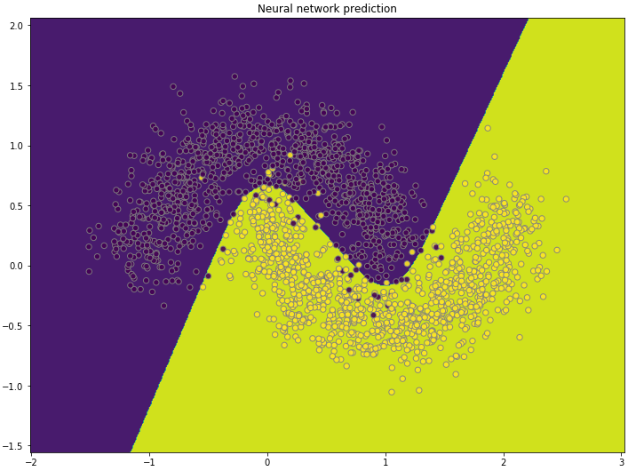 prediction boundary on moon dataset using neural network