DeepMind’s founder says to build better machine learning brain, we need to learn from neurosciences. “In both biological and artificial systems, successive non-linear computations transform raw visual input into an increasingly complex set of features, permitting object recognition that is invariant to transformations of pose, illumination, or scale.”
Table of Contents
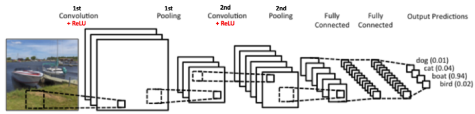
In this post, I will go over convolutional neural networks (CNNs) example using the MNIST dataset. Most of CNN examples on internet are quite complex with at least two convolutional layers, like the one below:
 From Wikipedia
Overview
I will write python script sequentially using only a single layer of convolution, step by step with a piece of code to peek the Tensorflow graph and intermediate results.
There are mainly four steps:
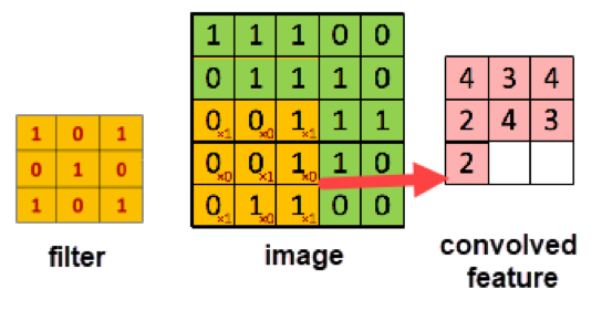
- Convolution: extract features from the input image using filter. Each pixel of convoluted feature image is a linear combination of multiple nearby (in 3 by 3, or 5 by 5 matrix) pixels of the original image. The linear combination matrix applied on the in 3 by 3, or 5 by 5 matrix is called filter. It is the same filter we usually called in Adobe Photoshop or Picasa, which help us sharpen or blur images. The values used for filter will be learned from training set.
- Non linear activation: ReLU is usually used since it is found to be better in most cases. ReLU change all negative values in feature matrix to be zeros. ReLU introduce non-linearity after the linear operation of the convolution step.
- Pooling or Sub Sampling: pooling reduces the dimension of feature image to smaller scale. Max pooling is usually used which takes the largest value in the 2*2 (or other predefined) window in the feature image. Pooling reduces the dimension of data and reduces the number of parameters to be learnt/trained.
- Classification: it is a step to flatten the image and feed to regular neural network with two hidden layers, and usually use softmax to get final output.
Step 1: setup MNIST dataset input placeholders
import sys
import tensorflow as tf
import numpy as np
from tensorflow.examples.tutorials.mnist import input_data
import matplotlib.pyplot as plt
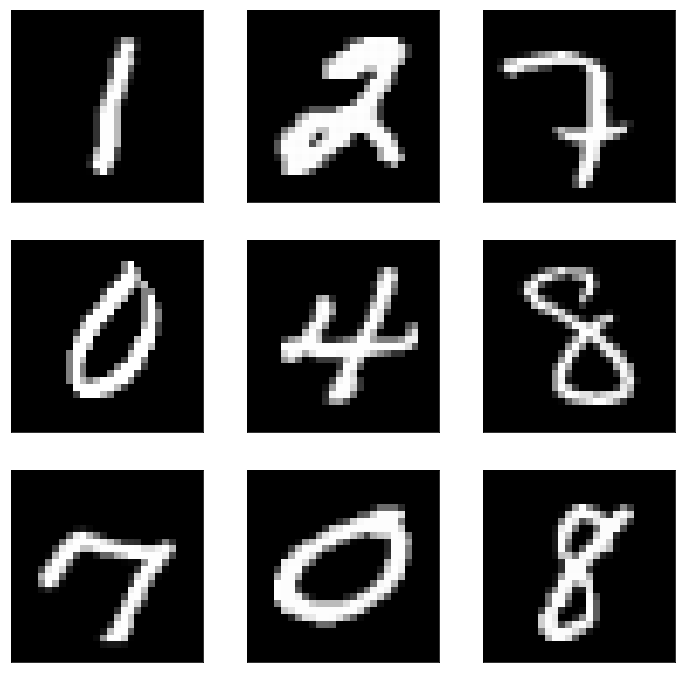
mnist = input_data.read_data_sets("A:\\Documents\\MNIST_data\\", one_hot=True);
batch_x, batch_y = mnist.train.next_batch(batch_size=10)
learning_rate = 0.0001
epochs = 10
batch_size = 50
# declare the training data placeholders
x = tf.placeholder(tf.float32, [None, 784], name='x')
# now declare the output data placeholder - 10 digits
y = tf.placeholder(tf.float32, [None, 10], name='y_true')
x_shaped = tf.reshape(x, [-1, 28, 28, 1], name='x_shaped')
The script above get the MNIST dataset and create placeholders in Tensorflow
- x, which has a vector with length 784 = 28 x 28 for each image. It is the flattened image data that is drawn from function mnist.train.nextbatch(). I draw one batch to get examples of placeholders using peek code below.
- Y, which is the final possible prediction outputs: 0, 1, …, 9
- We can reshape x to have dimension
[-1, 28, 28, 1]. The first value (-1) tells function to dynamically shape based on the amount of data passed to it. The 28*28 dimension are set for image size, and the last dimension 1 is for channel. For image with RGB, there three channels; for MINIST data with grey scale, it only has one channel.
We can peek the layout by run a TensorFlow session and get x_shaped as output from the session:
sess = tf.Session()
x_test, y_test = sess.run([x_shaped, y], feed_dict={x: batch_x, y: batch_y})
sess.close()

import matplotlib
%matplotlib inline
matplotlib.rcParams['figure.figsize'] = (12.0, 12.0)

print(np.shape(x_test[0, :, :, 0]))
f, ax = plt.subplots(3, 3)
k = 0;
for i in range(3):
    for j in range(3):
        ax[i, j].matshow(x_test[k, :, :, 0], cmap='gray')
        ax[i, j].set_title('')
        ax[i, j].set_xticks([])
        ax[i, j].set_yticks([])
        k += 1

plt.show();
Step 2: Create convolution layer with filter
Full code with old codes greyed and new codes colored:
import sys
import tensorflow as tf
import numpy as np
from tensorflow.examples.tutorials.mnist import input_data
import matplotlib.pyplot as plt

mnist = input_data.read_data_sets("A:\\Documents\\MNIST_data\\", one_hot=True);

batch_x, batch_y = mnist.train.next_batch(batch_size=10)
learning_rate = 0.0001
epochs = 10
batch_size = 50

# declare the training data placeholders
x = tf.placeholder(tf.float32, [None, 784], name='x')
# now declare the output data placeholder - 10 digits
y = tf.placeholder(tf.float32, [None, 10], name='y_true')
x_shaped = tf.reshape(x, [-1, 28, 28, 1], name='x_shaped')
# create a single layer with 32 filters with size 5*5
name="layer1"
num_input_channels=1
num_filters=32
filter_shape=[5, 5]
conv_filt_shape = [filter_shape[0], filter_shape[1], num_input_channels, num_filters]

# initialize weights and bias for the filter conv_filt_shape = [5, 5, 1, 32]
weights = tf.Variable(tf.truncated_normal(conv_filt_shape, stddev=0.03)
                                                     , name=name+'_W')
bias = tf.Variable(tf.truncated_normal([num_filters]), name=name+'_b')

# input: [batch, in_height, in_width, in_channels]
# filter: [filter_height, filter_width, in_channels, out_channels]
# strides: move step on each direction
out_layer_conv = tf.nn.conv2d(input=x_shaped,
                             filter=weights,
                            strides=[1, 1, 1, 1],
                            padding='SAME', name=name+'_cov1')
- Input is a 4-D tensor with dimension: [-1, 28, 28, 1], [batch, in_height, in_width, in_channels]
- Filter has size 5 x 5 and we move the 5 x 5 window on the images to get convolutional feature map. In total, 32 filters are specified and initialized with value in weights/bias to be trained. The filter/weight dimension is [5, 5, 1, 32], [filter_height, filter_width, in_channels, out_channels], so for input image pixel values in filter window [-1, 5, 5, 1]* [5, 5, 1, 32] will have dimension [-1, 32], outputting 32 values for each input image from 32 filters.
- Strides specify the window moving steps with one step on each direction.
- Padding specify padding choice we can use for pixels on image boundaries. Option “SAME” will pad evenly left and right and extra column is added to the right if necessary.
- The convolutional output is dimension [-1, 28, 28, 32]
We can peek the TensorFlow graph by session run below to get output layer:
init_op = tf.global_variables_initializer()
sess=tf.Session()
sess.run(init_op)
# input the first batch, and get output
x_c, w_c, b_c, o_c = sess.run([x_shaped, weights, bias, out_layer_conv],
                              feed_dict={x: batch_x, y: batch_y})
sess.close()
print(np.shape(x_c)); print(np.shape(w_c));
print(np.shape(b_c)); print(np.shape(o_c));
# check the first filter window on first image
print(x_c[0, 10:15, 10:15, 0]);
# print the first filter used for first output channel
print(w_c[0:5, 0:5, 0, 0]);
# mutiple pixels in image window with filter weights
print(np.multiply(w_c[0:5, 0:5, 0, 0], x_c[0, 10:15, 10:15, 0]));
print(np.sum(np.multiply(w_c[0:5, 0:5, 0, 0], x_c[0, 10:15, 10:15, 0])));
# The value should be the same as the output value from out_layer_conv
# with SAME padding (padding 2 on all directions)
print(o_c[0, 12, 12, 0])
(5, 5, 1, 32)

(32,)

(10, 28, 28, 32)

[[ 0.          0.          0.          0.          0.1254902 ]
 [ 0.          0.          0.          0.          0.36078432]
 [ 0.          0.10980393  0.1254902   0.36078432  0.92549026]
 [ 0.25098041  0.92549026  0.98431379  0.99215692  0.98431379]
 [ 0.37254903  0.95686281  0.98431379  0.99215692  0.98431379]]

[[ 0.03758693 -0.01360717  0.01783204  0.02611525  0.0352986 ]
 [-0.01341566  0.01930063  0.01323777  0.00718748  0.00588328]
 [ 0.00498071  0.00780649 -0.01162758 -0.02254303 -0.01474185]
 [-0.01541197 -0.04706075 -0.0072391   0.02696476  0.00126157]
 [ 0.01467456  0.00673592  0.04502914  0.0115862  -0.02767358]]

[[ 0.         -0.          0.          0.          0.00442963]
 [-0.          0.          0.          0.          0.0021226 ]
 [ 0.          0.00085718 -0.00145915 -0.00813317 -0.01364344]
 [-0.0038681  -0.04355427 -0.00712555  0.02675327  0.00124178]
 [ 0.00546699  0.00644535  0.0443228   0.01149533 -0.02723948]]

-0.00188821

-0.00188822
As the ouput print show,
- x_shaped has dimension [10, 28, 28, 1] for the first batch of 10 images.
- Filter weight dimension is [5, 5, 1, 32]
- The output feature image is also [10, 28, 28, 1] since we slide only one on all four dimension and we padded all four boundaries.
- The np.multiply(w_c[0:5, 0:5, 0, 0], x_c[0, 10:15, 10:15, 0]) which multiply each pixel values in [10:15, 10:15] of the first image (digit 9) with first filter weight, the value is the same as tf.nn.conv2d output on first channel output on position [12, 12] since we padded boundaries with 2 columns/rows (for filter size 5 x 5).
Step 3: max pooling
Full code with old codes greyed and new codes colored:
import sys
import tensorflow as tf
import numpy as np
from tensorflow.examples.tutorials.mnist import input_data
import matplotlib.pyplot as plt

mnist = input_data.read_data_sets("A:\\Documents\\MNIST_data\\", one_hot=True);

batch_x, batch_y = mnist.train.next_batch(batch_size=10)
learning_rate = 0.0001
epochs = 10
batch_size = 50

# declare the training data placeholders
x = tf.placeholder(tf.float32, [None, 784], name='x')
# now declare the output data placeholder - 10 digits
y = tf.placeholder(tf.float32, [None, 10], name='y_true')
x_shaped = tf.reshape(x, [-1, 28, 28, 1], name='x_shaped')

# create a single layer with 32 filters with size 5*5
name="layer1"
num_input_channels=1
num_filters=32
filter_shape=[5, 5]
conv_filt_shape = [filter_shape[0], filter_shape[1], num_input_channels, num_filters]

# initialize weights and bias for the filter conv_filt_shape = [5, 5, 1, 32]
weights = tf.Variable(tf.truncated_normal(conv_filt_shape, stddev=0.03),
                                                       name=name+'_W')
bias = tf.Variable(tf.truncated_normal([num_filters]), name=name+'_b')

# input: [batch, in_height, in_width, in_channels]
# filter: [filter_height, filter_width, in_channels, out_channels]
# strides: move step on each direction
out_layer_conv = tf.nn.conv2d(input=x_shaped,
                             filter=weights,
                            strides=[1, 1, 1, 1],
                            padding='SAME', name=name+'_cov1')
# add the bias
out_layer_add_bias = tf.add(out_layer_conv, bias, name=name+"_bias")
# apply a ReLU non-linear activation
out_layer_relu = tf.nn.relu(out_layer_add_bias, name=name+"_RELU")

# now perform max pooling
pool_shape=[2, 2]
# ksize is the argument which defines the size of the max pooling window
ksize = [1, pool_shape[0], pool_shape[1], 1]
# strides defines how the max pooling area moves through the image
strides = [1, 2, 2, 1]
out_layer1 = tf.nn.max_pool(out_layer_relu, ksize=ksize,
                            strides=strides, padding='SAME',
                            name=name+"_Maxpool");
- Add bias for each channel after applying its filter, then apply ReLU for non-linearity
- Input for max pool is a 4-D tensor with dimension: [-1, 28, 28, 32], [batch, in_height, in_width, out_channels]
- The max pool using size 2*2 to get the max values from neighborhood of 4 feature values. The stride is [1, 2, 2, 1] so it moves every two positions within the image feature and do not move outside of image for max pooling (do not max pooling across multiple channels). Since it moves every two positions, the output has dimension [-1, 14, 14, 32]
We can peek the TensorFlow graph by session run below to get reduced layer after max pooling:
init_op = tf.global_variables_initializer()
sess=tf.Session()
sess.run(init_op)
b_c, r_c, o_c = sess.run([out_layer_add_bias, out_layer_relu, out_layer1],
                                       feed_dict={x: batch_x, y: batch_y})
sess.close()
print(np.shape(b_c)); print(np.shape(r_c)); print(np.shape(o_c));
i=6; srt=2*i; end=2*(i+1)
print(b_c[1, srt:end, srt:end, 5]);
print(r_c[1, srt:end, srt:end, 5]);
print(o_c[1, i, i, 5]);
(10, 28, 28, 32)

(10, 28, 28, 32)

(10, 14, 14, 32)

[[ 0.62240434  0.63935971]
 [ 0.6250062   0.64221692]]

[[ 0.62240434  0.63935971]
 [ 0.6250062   0.64221692]]

0.642217
The max of 2*2 matrix in [12:14, 12:14] is 0.6422. Here all bias values are still zeros since it has not been trained yet.
Step 4: classification using NN
Full code with old codes greyed and new codes colored:
import sys
import tensorflow as tf
import numpy as np
from tensorflow.examples.tutorials.mnist import input_data
import matplotlib.pyplot as plt

mnist = input_data.read_data_sets("A:\\Documents\\MNIST_data\\", one_hot=True);

batch_x, batch_y = mnist.train.next_batch(batch_size=10)
learning_rate = 0.0001
epochs = 10
batch_size = 50

# declare the training data placeholders
x = tf.placeholder(tf.float32, [None, 784], name='x')
# now declare the output data placeholder - 10 digits
y = tf.placeholder(tf.float32, [None, 10], name='y_true')
x_shaped = tf.reshape(x, [-1, 28, 28, 1], name='x_shaped')

# create a single layer with 32 filters with size 5*5
name="layer1"
num_input_channels=1
num_filters=32
filter_shape=[5, 5]
conv_filt_shape = [filter_shape[0], filter_shape[1], num_input_channels, num_filters]

# initialize weights and bias for the filter conv_filt_shape = [5, 5, 1, 32]
weights = tf.Variable(tf.truncated_normal(conv_filt_shape, stddev=0.03),
                                                        name=name+'_W')
bias = tf.Variable(tf.truncated_normal([num_filters]), name=name+'_b')

# [batch, in_height, in_width, in_channels]
out_layer_conv = tf.nn.conv2d(input=x_shaped,
filter=weights, # [filter_height, filter_width, in_channels, out_channels]
strides=[1, 1, 1, 1], # move step on each direction
padding='SAME', name=name+'_cov1')

# add the bias
out_layer_add_bias = tf.add(out_layer_conv, bias, name=name+"_bias")
# apply a ReLU non-linear activation
out_layer_relu = tf.nn.relu(out_layer_add_bias, name=name+"_RELU")

# now perform max pooling
pool_shape=[2, 2]
# ksize is the argument which defines the size of the max pooling window
ksize = [1, pool_shape[0], pool_shape[1], 1]
# strides defines how the max pooling area moves through the image
strides = [1, 2, 2, 1]
out_layer1 = tf.nn.max_pool(out_layer_relu, ksize=ksize, strides=strides,
                                   padding='SAME', name=name+"_Maxpool")
# flatten the output max pooled feature from all 32 channels
flattened = tf.reshape(out_layer1, [-1, 14 * 14 * 32])

# setup some weights and bias values for first dense layer with 1000 nodes, then activate with ReLU
wd1 = tf.Variable(tf.truncated_normal([14 * 14 * 32, 1000], stddev=0.03), name='wd1')
bd1 = tf.Variable(tf.truncated_normal([1000], stddev=0.01), name='bd1')
dense_layer1 = tf.add(tf.matmul(flattened, wd1), bd1, name="dense1")
dense_layer1_relu = tf.nn.relu(dense_layer1, name="dense1_RELU")

# another layer to output with final 10 nodes and use softmax activations for prediction
wd2 = tf.Variable(tf.truncated_normal([1000, 10], stddev=0.03), name='wd2')
bd2 = tf.Variable(tf.truncated_normal([10], stddev=0.01), name='bd2')
dense_layer2 = tf.add(tf.matmul(dense_layer1_relu, wd2), bd2, name="dense_layer2")
y_ = tf.nn.softmax(dense_layer2, name="predict_y")

cross_entropy = tf.reduce_mean(tf.nn.softmax_cross_entropy_with_logits(logits=dense_layer2, labels=y)
                                                         , name="cross_entropy")

# add an optimiser
optimiser = tf.train.AdamOptimizer(learning_rate=learning_rate).minimize(cross_entropy)

# define an accuracy assessment operation
correct_prediction = tf.equal(tf.argmax(y, 1), tf.argmax(y_, 1), name="accuracy_check")
accuracy = tf.reduce_mean(tf.cast(correct_prediction, tf.float32), name="accuracy")

# setup the initialisation operator
init_op = tf.global_variables_initializer()

# setup recording variables
# add a summary to store the accuracy
tf.summary.scalar('accuracy', accuracy)
tf.summary.scalar('cross_entropy', cross_entropy)
merged = tf.summary.merge_all()
writer = tf.summary.FileWriter('/Users/gary.ge/Dropbox/codespace/com.fg.python/src/examples/tensorboard/ts03')

epochs = 10
with tf.Session() as sess:
    # initialise the variables
    sess.run(init_op)
    total_batch = int(len(mnist.train.labels) / batch_size)
    writer.add_graph(sess.graph);
    for epoch in range(epochs):
        avg_cost = 0
        for i in range(total_batch):
            batch_x, batch_y = mnist.train.next_batch(batch_size=batch_size)
            _, c = sess.run([optimiser, cross_entropy], feed_dict={x: batch_x, y: batch_y})
            avg_cost += c / total_batch
        test_acc = sess.run(accuracy, feed_dict={x: mnist.test.images, y: mnist.test.labels})
        print("Epoch:", (epoch + 1), ", cost =", "{:.3f}".format(avg_cost), " test accuracy: {:.3f}".format(test_acc))
        summary = sess.run(merged, feed_dict={x: mnist.test.images, y: mnist.test.labels})
        writer.add_summary(summary, epoch)

    print("\nTraining complete!")
    final_accuracy, input_shaped, out_layer_conv, out_layer_relu, output_layer1, dense1, dense2 = sess.run([accuracy, x_shaped, out_layer_conv, out_layer_relu, out_layer1, dense_layer1, dense_layer2], feed_dict={x: mnist.test.images, y: mnist.test.labels})
    print(final_accuracy)
Epoch: 1 , cost = 0.779  test accuracy: 0.900
Epoch: 2 , cost = 0.292  test accuracy: 0.932
Epoch: 3 , cost = 0.213  test accuracy: 0.948
Epoch: 4 , cost = 0.158  test accuracy: 0.956
Epoch: 5 , cost = 0.125  test accuracy: 0.972
Epoch: 6 , cost = 0.101  test accuracy: 0.971
Epoch: 7 , cost = 0.085  test accuracy: 0.978
Epoch: 8 , cost = 0.074  test accuracy: 0.977
Epoch: 9 , cost = 0.066  test accuracy: 0.980
Epoch: 10 , cost = 0.058  test accuracy: 0.983

Training complete!
0.9828
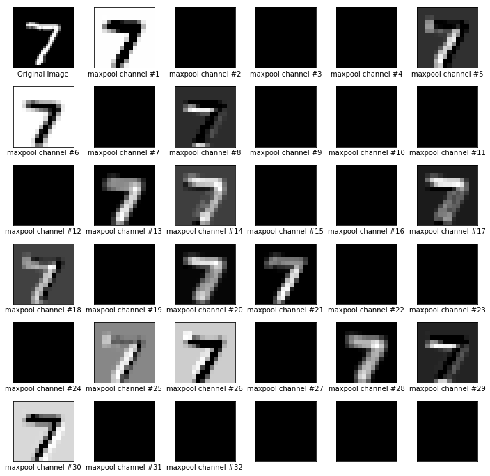
For each original 2828 image, we get 2828 convoluted features with 32 channels, and then get 1414 max pooled features with 32 channels. We reshape the [14, 14, 32] matrix to a 1414*32 single vector for each original image, and use it as input for neural network with 1000 hidden nodes and 10 output nodes.
The final softmax function will predict the final digit from the image, and the prediction accuracy is defined as the average of True/False of all digit predictions.
In the final session run, we used 10 epochs, and run though all mini batches (batch size 50 images) in each epoch. The accuracy has been assessed in each epoch, and it has been improved with final accuracy 98.28%. It is a pretty good result using a single layer of convolution. You can further improve it with a second convolutional layer.
After all epochs are finished, we finished the training for CNN. I get the final estimate of all intermediate values: input_shaped, out_layer_conv, out_layer_relu, output_layer1, dense1, dense2. We can further visualize how it looks like in these layers.
First, we define a plot function to plot the original digit image along with images from all 32 channels after convolution, ReLU and maxpool:
def plot_original_and_layer(nrow, ncol, mat_ori, mat_layers, tag):
    fig, axes = plt.subplots(nrow, ncol)
    fig.subplots_adjust(hspace=0.3, wspace=0.3)

    for i, ax in enumerate(axes.flat):
        # Plot image
        if (i == 0):
            ax.imshow(mat_ori, cmap='gray')
            xlabel = "Original Image"
        elif (i <= 32):
            ax.imshow(mat_layers[:, :, i-1], cmap='gray')
            xlabel = tag+" channel #{0}".format(i)
        else:
            ax.imshow(np.zeros(np.shape(mat_ori)), cmap='gray')
            xlabel = ""

        ax.set_xlabel(xlabel)
        # Remove ticks from the plot.
        ax.set_xticks([])
        ax.set_yticks([])
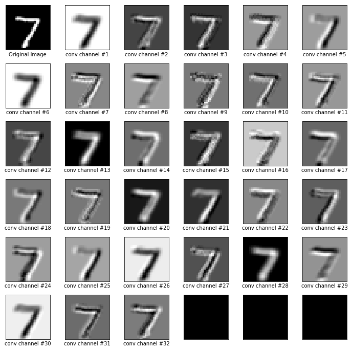
Plot digit image along with images from all 32 channels after convolution:
image_index=0
import matplotlib
%matplotlib inline
matplotlib.rcParams['figure.figsize'] = (12.0, 12.0)
# visulize the covlutional layer
plot_original_and_layer(6, 6, input_shaped[image_index, :, :, 0],
                                  out_layer_conv[image_index, :, :, :], "conv")
plt.show()
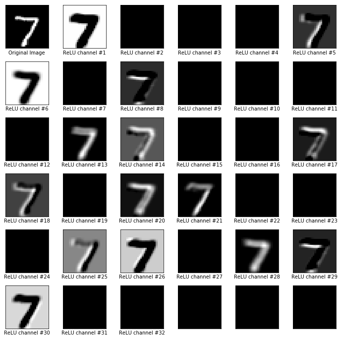
Plot digit image along with images from all 32 channels after convolution and ReLU:
# visulize the ReLU layer
plot_original_and_layer(6, 6, input_shaped[image_index, :, :, 0], out_layer_relu[image_index, :, :, :], "ReLU")
Plot digit image along with images from all 32 channels after convolution, ReLU and maxpool:
# Visulize the feature images after maxpool
plot_original_and_layer(6, 6, input_shaped[image_index, :, :, 0], output_layer1[image_index, :, :, :], "maxpool")
We can also check the final 10 values in second dense layer, and its probabilities for number 0, 1, 2…, 9
# visulize the final 0-9 prediction before and after softmax
dense2_array = dense2[image_index, :];
def softmax(x):
    """Compute softmax values for each sets of scores in x."""
    e_x = np.exp(x - np.max(x))
    return e_x / e_x.sum()

print("dense layer #2")
print(dense2_array)
print("probabilities for number 0, 1, 2..., 9")
print(softmax(dense2_array))
dense layer #2
[ -2.46648407  -6.44926643   1.21165502   2.62235379  -7.3579154
  -3.27135062 -13.57719803  11.59324932  -1.48232484  -0.61677217]
probabilities for number 0, 1, 2..., 9
[  7.83182713e-07   1.45936232e-08   3.09926327e-05   1.27033185e-04
   5.88222582e-09   3.50198206e-07   1.17095691e-11   9.99833584e-01
   2.09545397e-06   4.97946394e-06]
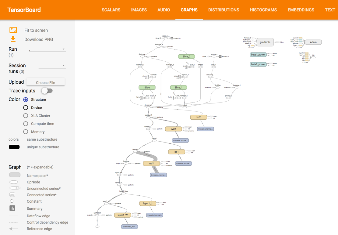
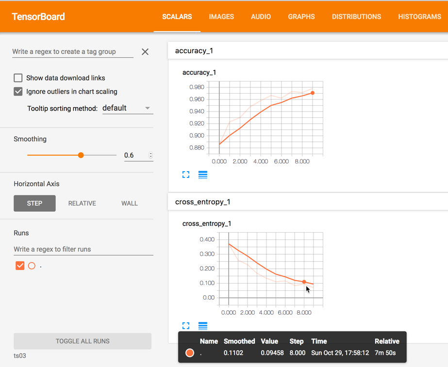
TensorBoard
We can also take a look at the tensorboard since we labelled most variables with names.
cd A:\Documents
tensorboard --logdir="tensorboard"
Check the scalar and graph tab: